Where Inference Runs Is a Cost Decision, and the Crossover Runs Both Ways
Hourly accelerator prices are the wrong unit for deciding where self-hosted inference runs. Measured as cost per useful answer, central placement wins for large, batchable work and distributed placement for small, latency-bound, payload-heavy work. Utilisation decides most cases.
Audio edition
Read by a synthetic voice cloned from John with his consent. About the audio edition
The price of an accelerator-hour tells you almost nothing about where inference should run. Two deployments of the same model on the same hardware can differ several-fold in what each delivered answer costs, and the difference comes from things the hourly price leaves out: how busy the hardware is, how much data has to travel to reach it, and how many answers arrive too late to be any use. Placement is a cost decision, and the crossover between central and distributed placement runs in both directions.
That second half is the part most arguments about inference placement skip. The case for putting inference close to users is real for some workloads. For others, a central region is cheaper by a wide margin and no amount of latency argument changes that. The useful position is knowing which variables flip it.
This post sits between three others. AI Cost Curves answers whether to call an API or run the model yourself. Model Routing answers which model should take each request. The AI Grid describes the tiered architecture. This one assumes you have already decided to self-host a given model, and asks where it should sit and what each answer costs there.
What the hourly price hides
An hourly or per-token price is a price for capacity. What you want to buy is answers, and four things sit between the two.
Utilisation. An accelerator you pay for and do not use still costs the full hour. A central region pools demand from every user and every time zone into one place, so the peaks of one population fill the troughs of another. A distributed footprint splits that demand across many locations, and each location has to be sized for its own local peak. The aggregate traffic is identical. The average utilisation per location is lower, because each site carries its own headroom.
Batching. Inference throughput on a modern accelerator rises sharply when requests are batched together, and batching needs a queue deep enough to fill a batch without making anyone wait long. Pooled demand gives you that queue. A small site serving a thin slice of traffic often does not, so it runs smaller batches and gets fewer answers per hour from the same hardware. This effect grows with model size.
Data movement. Every request has to get its input to the model and its output back. For a text prompt and a text answer, that is a few kilobytes and the cost is negligible. For a camera frame, an audio stream or a document scan, it can be orders of magnitude more, and moving it to a central region and back is a recurring cost that the hourly price never shows. The glossary defines egress fees, which is where this line item usually surfaces.
Late answers. An answer that arrives after the user has given up, after the video frame has rendered or after the transaction has been approved without it has cost the full price and delivered nothing. For latency-tolerant work this rate is close to zero wherever the model sits. For latency-bound work it depends on distance, and it is the one cost that falls as you move closer to users.
There is a fifth cost, which is operational: every location is something to deploy to, patch, monitor and roll back. I leave it out of the arithmetic below because it varies more by team than by workload, but it belongs in any real comparison and it always counts against more locations.
Cost per useful answer
The unit I use is cost per useful answer: what you spend, divided by the answers that arrived inside the latency budget the product actually has.
cost per useful answer =
  (capacity cost ÷ utilisation  +  data movement per request)
  ÷ share of answers inside the latency budget
None of the four terms is exotic. Most teams can estimate all of them from data they already have. What is unusual is putting them in one expression, because each term usually belongs to a different person: capacity to the platform team, data movement to whoever owns the network bill, and the late-answer rate to the product team, if anyone measures it at all.
A worked example, with illustrative numbers
Every number in this section is illustrative, priced in made-up relative units to show the shape of the calculation. None comes from a real price list, provider or workload. Substitute your own.
Take one small model and compare two placements. Each figure is per 1,000 requests.
- Capacity. Serving 1,000 requests on fully used hardware costs 10 units in a central region. In a distributed footprint I assume 12.5 units, a 25% premium, on the reasoning that small sites rarely buy power, cooling and hardware at the density of large ones. If your numbers show no premium, the distributed case improves.
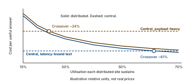
- Utilisation. The central region runs at 60%, helped by pooling and batching. Distributed sites run at whatever their local demand supports, which is the variable on the chart below.
- Data movement. A text workload costs 1 unit in either placement. A payload-heavy workload, say images or audio sent upstream, costs 30 units to haul to a central region and 5 to handle locally.
- Useful answers. For latency-bound work, I assume 80% of centrally served answers land inside the budget against 97% of locally served ones. For latency-tolerant work, both placements deliver 100%.
Run those through the formula:
| Workload (illustrative) | Central | Distributed at 30% utilisation | Distributed at 60% utilisation |
|---|---|---|---|
| Small model, latency-tolerant text | 17.7 | 42.7 | 21.8 |
| Small model, latency-bound text | 22.1 | 44.0 | 22.5 |
| Small model, latency-bound, payload-heavy | 58.3 | 48.1 | 26.6 |
Three readings, and they hold whatever numbers you substitute.
In this example, latency on its own does not pay for distribution. In the second row, the central placement loses one answer in five to the latency budget and still costs about the same as a distributed footprint running at 60%. At a more typical 30%, distribution costs twice as much. Latency has to be expensive before it decides the question by itself.
Data movement moves the crossover further than anything else. In the third row, the same model with heavy payloads is cheaper distributed even at 30% utilisation. The hourly price did not change. What changed is that every centrally served request now carries a haulage charge that a local one avoids.
Utilisation is the distributed footprint’s whole problem. Every distributed figure improves sharply as utilisation rises, and the central figure does not move at all. A distributed placement that cannot keep its sites busy is buying latency with idle hardware.
When central placement wins
Central or regional placement is the cheaper answer more often than the latency argument alone suggests. It wins when:
- The model is large. Large models need more memory than a small site usually provides, and they gain the most from batching, which needs pooled demand. A large model spread thinly across many sites pays for the hardware many times and batches poorly everywhere.
- The work is batchable. Overnight document processing, embedding generation, evaluation runs and back-office classification have no user waiting. The late-answer term is zero, so the only argument for distribution disappears, and a central queue can run at utilisation no distributed footprint will match.
- The request rate is low or uneven. A workload with a few thousand requests a day cannot keep even one site busy, let alone many. Below that threshold, every additional location is mostly idle capacity.
- The data already lives centrally. If each request reads from a large corpus, a vector index or a transactional store that sits in one region, moving the model away from that data turns a local read into a long-distance one on every request. Data gravity works against distribution as often as for it, and it is also where the residency questions in Data Residency Is Not Sovereign AI tend to land.
When distributed placement wins
Distributed placement wins on a narrower set of conditions, and it wins decisively when they line up:
- The model is small. A quantised model of a few billion parameters fits modest hardware, and model compression is what makes it viable at all. The smaller the model, the smaller the utilisation penalty per site.
- The latency budget is tight and enforced. Where an answer outside the budget is worthless, the late-answer term becomes large for a distant model. A tolerance of seconds does not count; a frame budget or a conversational turn does.
- Fan-out is high. Interactive features that call a model several times per user action multiply every round trip. An extra 80 milliseconds (an illustrative figure) is tolerable once and not five times in sequence.
- The payload is heavy and the answer is light. Images, audio and sensor data in, a short classification or decision out. This is the case the illustrative table shows most clearly, and it is where the crossover arrives at the lowest utilisation.
- Demand is dense enough per location. The distributed case improves faster with per-site volume than with anything else. Markets with concentrated users can sustain it where sparse ones cannot.
Most estates have workloads on both lists. That is the expected result, and it is why the AI Grid insight describes tiers and a routing decision between them rather than a single location.
Where the curve bends
Four variables move the crossover, and each one can be measured before any placement decision is made:
- Achievable utilisation per site, which follows from the per-location request rate and the shape of its daily peak. This is the variable that decides most cases, and it is the one most often assumed rather than measured.
- Data moved per request, in each direction. Text workloads barely register here. Media and sensor workloads dominate everything else in the formula.
- The late-answer rate at each distance, measured against the budget the product actually enforces, not the one in the design document.
- Model size, which sets both the hardware floor per site and how much the workload gains from central batching.
Geography acts through the first and third. Moving the same workload to a market with more dispersed users lowers per-site utilisation and raises the late-answer rate for a central placement at the same time, which is why a placement that is right in one region can be wrong in the next.
The test I apply
Before anyone argues for a placement, I ask for one number per candidate: the cost per useful answer at the utilisation the placement will really achieve. Not the utilisation on the capacity plan, and not the hourly price. If the team cannot produce it, the first piece of work is measurement, not migration: a week of per-location request rates, payload sizes in both directions and the share of answers that land inside the latency budget.
Most of the time that week settles the question. Large, batchable, text-shaped work stays central and should. Small, latency-bound, payload-heavy work moves out and should. The workloads in between are where the arithmetic is close, and close arithmetic is an argument for keeping the placement decision reversible, not for making it once.
For the step before this one, read AI Cost Curves and the interactive framework. For deciding which model takes each request, read Model Routing. For the tiered architecture and its routing calculator, see The AI Grid.
Source: https://bradshaw.cloud/writing/inference-placement-crossover/